At profiq, we are always interested in learning something new, and trying novel technologies. One of these technologies is Elixir—a functional programming language whose main strengths lie in fault tolerance and scalability through concurrency. This makes it a good candidate for backend development, especially when it comes to high-traffic web applications. We, for example, utilize Elixir’s properties in cooperation with Divvy to handle a large number of financial transactions. But, this, of course, is not its only use. As it turns out, Elixir can do a lot more. One of the most interesting applications, we discovered, is in deep learning.

In this article, we will show you the deep learning tools Elixir offers, and how you can use these tools to implement, train, and evaluate a simple convolutional neural network for image classification.

Note: This article was edited on November 12, 2021 to reflect latest changes in Axon’s and EXLA’s APIs.

Why consider Elixir for deep learning?

Most data scientists and machine learning (ML) specialists use Python. And, no wonder. This language is relatively easy to learn and use even for people whose main focus is not software development. Python also offers many libraries for scientific computing, data analysis, or deep learning. And, the use cases do not end there. It is a programming language intended for general use. So, if you want to wrap your ML model or the results of your research into a web or desktop application, you can do so easily with Python.

So, why bother with looking for other solutions? Just as pretty much every tool does, Python, too, has its disadvantages. The most notable one is speed. Most data science and ML frameworks are at least partly written in lower-level languages such as C or C++. By themselves, these tools are usually as fast as it gets. But, performance issues might occur when you have to write a more complex routine directly in Python; for example, a data preprocessing pipeline. In such cases, the performance limitations become quite apparent. Python is also not the best tool for parallel programming. Because of its

global interpreter lock

(GIL), the use of multithreading is very limited. GIL is one of the reasons why many data scientists look for alternatives. Using processes instead of threads is possible, but there is a lot of overhead, and issues with sharing data between processes arise quite often.

This last disadvantage is why Elixir could be considered a suitable alternative for deep learning applications—it is built with concurrency in mind. Other potential advantages might arise from differences in paradigms. Elixir is a functional programming language and uses immutable types. This mitigates the amount of issues caused by unexpected data structure manipulations. Other benefits often presented by proponents of functional programming include better testability or higher level of abstraction, which leads to easier comprehension. For a more detailed description of differences between Python and Elixir, we refer you to this

Elixir forum discussion thread

.

The toolbox

Unless you are a masochist and decide to implement everything from scratch, you can’t do much deep learning out-of-the-box without installing some additional libraries and tools. This is true for both Elixir and Python. So, which libraries make deep learning in Elixir possible?

The basic building block of the whole Elixir deep learning stack is

Nx

. Nx is a library for working with multidimensional arrays. It is a bit similar to Numpy, but a more suitable analogy might be PyTorch or Tensorflow, but without deep learning. Nx lets you define tensors and perform algebraic operations. And, thanks to an optional integration with Google’s XLA compiler through

EXLA

, all these operations can be performed on a GPU.

Axon

is a library built on top of Nx. It provides a high-level API for neural network definition, training, and evaluation. To use an analogy from the world of Python, Axon is pretty similar to Keras.

The final component of our deep learning stack is

Livebook

. This tool should be very familiar to those who use Jupyter Notebook. Livebook is simply a Jupyter alternative for Elixir that lets you do all the good stuff you would expect: running a simple IDE in a web browser, interactive computing by splitting your code into multiple cells that can be evaluated separately on demand, or providing additional markdown documentation to your code.

What gives this toolbox a lot of credibility is the fact that even José Valim—the author of Elixir— contributes to its development.

The problem

To show you how these tools can be used to define and train an ML model, we will solve a simple image classification problem. Using a publicly available

dataset

from Kaggle, we will train a model for recognizing pneumonia from an x-ray image. We will consider only two possible classes: class “1” labels images showing pneumonia while class “0” labels images without pneumonia.

To give you a visual sense of this classification problem, take a look at these two pictures. Assuming you are not a medical specialist, would you be able to determine which of these two pictures shows pneumonia and which one shows healthy lungs?

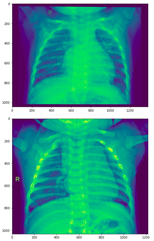
It turns out that the first image is an example of a patient with pneumonia while the second example shows healthy lungs.

Toolbox installation

We start our journey into deep learning in Elixir by installing all the tools we need. First, we of course need Elixir itself. If you don’t have Elixir on your machine, we recommend installing it using

asdf

. The installation process of EXLA also compiles TensorFlow from its source code. And, for that, you need

bazel

; specifically, in version 3.7.2. We again recommend using asdf for installation.

In our experiments, we installed the latest version of Livebook from its GitHub repository:

$ git clone https://github.com/elixir-nx/livebook.git
$ cd livebook
$ mix deps.get

Now, we can start the Livebook web server by executing:

$ mix phx.server

By default, the server runs on port 4000. You can open Livebook in your web browser by visiting

http://localhost:4000

.

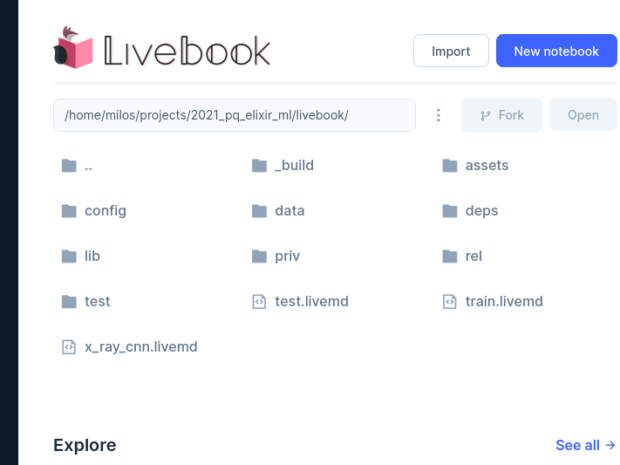
By clicking on

New notebook

, we can now create an empty interactive notebook, and name it

Pneumonia detection

.

We now create a new section by clicking on

+Section

. Sections help you structure your notebook. Each section has a title and can contain multiple cells. A cell represents a basic unit of notebook content. Livebook offers multiple types of cells such as

Markdown

for providing a nicely formatted commentary to your code, and

Elixir,

which contains pieces of executable code.

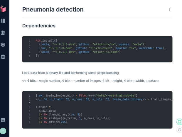
We create an Elixir cell and fill it with code for installing additional dependencies: Nx, EXLA, and Axon:

Mix.install([
  {:exla, "~> 0.1.0-dev", github: "elixir-nx/nx", sparse: "exla"},
  {:nx, "~> 0.1.0-dev", github: "elixir-nx/nx", sparse: "nx", override: true},
  {:axon, "~> 0.1.0-dev", github: "elixir-nx/axon"}
])

We can now evaluate the cell. Doing so for the first time can actually take several hours. As we already mentioned, TensorFlow is compiled from its source code during EXLA installation. This compilation takes a long time. EXLA installation can also be skipped if your goal is to just play with the code and don’t care too much about training and inference performance.

Loading data

All required dependencies are now installed. Now, we can load the data we will use to train and then test the model. We cheated a bit here and did a bit of preprocessing. Instead of having a filesystem directory containing all images as files, we created

four binary files

containing image data with unified size and labels split into training and test sets.

This data can be loaded into the Livebook environment with the following code:

{:ok, train_images_bin} = File.read("data/x-ray-train-ubyte")
<<_::32, n_train::32, n_rows::32, n_cols::32, train_data::binary>> = train_images_bin

Next, we create an Nx array from the binary data, reshape it into a multidimensional array with one dimension representing individual training samples, one dimension representing different color channels (in our case, we will be using only a single channel), and two dimensions representing rows and columns of individual pixels. Individual pixel values are then normalized, so 1 represents white and 0 represents black. Shades of grey are then represented by values between these two extremes:

x_train =
  train_data
  |> Nx.from_binary({:u, 8})
  |> Nx.reshape({n_train, 1, n_rows, n_cols})
  |> Nx.divide(255)

We can similarly load the labels for training data. The only difference will be in the last row. Instead of normalization, we one-hot encode our class labels:

{:ok, train_labels_bin} = File.read("data/x-ray-train-labels-ubyte")
<<_::32, n_labels::32, train_label::binary>> = train_labels_bin

y_test =
  test_label
  |> Nx.from_binary({:u, 8})
  |> Nx.reshape({n_test, 1})
  |> Nx.equal(Nx.tensor(Enum.to_list(0..1)))

After changing the file and variable names, the same process can be used to load the test data as well.

Nx also offers a helper function to split your data into batches for training and testing:

x = Nx.to_batched_list(x_train, batch_size)
y = Nx.to_batched_list(y_train, batch_size)

Defining and training a neural network

If you have experience with PyTorch or Keras, defining a neural network with Axon will be very natural to you. To solve our classification problem, we implemented a simple architecture with a few convolutional layers.

Convolution

is a technique proven to be very useful in image processing.

The following code snippet defines a neural network containing a sequence of four convolutional layers intertwined with so-called pooling layers. This convolution-pooling sequence is typical for image processing neural networks. Starting from very simple patterns such as vertical, diagonal, or horizontal lines, each layer can recognize more and more complex shapes. This sequence is then followed by three dense layers that, in short, take the different shapes recognized by the convolutional layers, and use them as features to classify the image. We also added a few dropout layers in between. These layers randomly “turn off” a small portion of neurons during training. It has been shown that this technique leads to better generalization (prediction on previously unseen data):

model =
  Axon.input({nil, 1, n_rows, n_cols})
  |> Axon.conv(16, kernel_size: {3, 3}, strides: 1, padding: :same, activation: :relu)
  |> Axon.max_pool(kernel_size: {2, 2}, strides: 2, padding: :same)
  |> Axon.conv(32, kernel_size: {3, 3}, strides: 1, padding: :same, activation: :relu)
  |> Axon.dropout(rate: 0.1)
  |> Axon.max_pool(kernel_size: {2, 2}, strides: 2, padding: :same)
  |> Axon.conv(32, kernel_size: {3, 3}, strides: 1, padding: :same, activation: :relu)
  |> Axon.dropout(rate: 0.1)
  |> Axon.max_pool(kernel_size: {2, 2}, strides: 2, padding: :same)
  |> Axon.conv(32, kernel_size: {3, 3}, strides: 1, padding: :same, activation: :relu)
  |> Axon.dropout(rate: 0.2)
  |> Axon.max_pool(kernel_size: {2, 2}, strides: 2, padding: :same)
  |> Axon.flatten()
  |> Axon.dense(16, activation: :relu)
  |> Axon.dropout(rate: 0.1)
  |> Axon.dense(8, activation: :relu)
  |> Axon.dense(2, activation: :softmax)

Training your model is again very straightforward. If you decide not to use EXLA, you can also skip the

compiler

parameter. But, in such cases, be ready for an extremely long training time:

trained_model =
  model
  |> Axon.Loop.trainer(:categorical_cross_entropy, Axon.Optimizers.adamw(0.000005))
  |> Axon.Loop.run(Stream.zip(x, y), epochs: epochs, compiler: EXLA)

Prediction and evaluation

We have trained our neural network. Now, we can use it to make a prediction—to classify a previously unseen image. To do so, we simply call the

Axon.predict/4

function:

result = Axon.predict(model, trained_model.params, x_test, compiler: EXLA)

Calling the function gives us a soft prediction, probabilities of our two classes. To make a hard prediction and decisively select one class, we can use the

Nx.argmax

function to choose the class with higher probability, with

Nx.reshape

and

Nx.equal

again one-hot encoding the result:

result =
  result
  |> Nx.argmax(axis: 1)
  |> Nx.reshape({624, 1})
  |> Nx.equal(Nx.tensor(Enum.to_list(0..1)))

Having both prediction results and test labels (loaded using the same procedure, as in the case of the training labels), we can now calculate different evaluation metrics, such as accuracy:

Axon.Metrics.accuracy(y_test, result)

After trying several configurations, we were able to reach accuracy of over 82% on testing data when using

AdamW optimizer

with the learning rate set to

0.000005,

training the network for 30 epochs.

Issues along the way

The Elixir machine learning stack is still quite new, and many things aren’t as polished as they could be. During our experiments, we encountered several issues.

The first issue is related to the choice of optimizer and loss function. We, for example, discovered that AdamW doesn’t work with binary cross entropy. That’s why we had to use categorical cross entropy, two output neurons, and one-hot encode the class labels.

The second important problem is GPU training and evaluation. Just like many other deep learning frameworks, the Axon, Nx, and EXLA support Nvidia GPUs through CUDA. But, setting up this GPU support is quite complicated. If you replicated all the steps we showed you so far, you might be disappointed to learn that everything is executed by your CPU, even though you might have a powerful GPU in your machine.

So, how to train your neural networks on a GPU? We started with a Google Cloud Engine VM with a Tesla T4. Our VM ran Ubuntu 20.04 with Nvidia drivers and CUDA 11.4 already installed. We then installed CuDNN 8.2.2 runtime using a DEB packaged downloaded from

CuDNN website

.

Next, instead of installing Axon, Nx and EXLA directly in a running Livebook instance, we added the dependencies to the

mix.exs

file:

defp deps do
  [
    {:phoenix, "~> 1.5"},
    ...
    {:bypass, "~> 2.1", only: :test},
    {:exla, "~> 0.1.0-dev", github: "elixir-nx/nx", sparse: "exla"},
    {:nx, "~> 0.1.0-dev", github: "elixir-nx/nx", sparse: "nx", override: true},
    {:axon, "~> 0.1.0-dev", github: "elixir-nx/axon"}
  ]
end

Then we downloaded and compiled the dependencies, setting the

XLA_TARGET

environment variable to

cuda111

(there was a small version missmatch, but everything seemed to work just fine):

$ mix deps.get
$ XLA_TARGET=cuda111 mix deps.compile

The step we struggled the most with was that even though EXLA is compiled with CUDA support, and you have CUDA and CUDNN installed, the CPU is still the default option for code execution. One of the ways to solve this problem is to change the default device inside the

config

/

config.exs

file by adding the following lines:

config :exla, :clients,
  default: [platform: :cuda]

Then we started the webserver:

ELIXIR_ERL_OPTIONS="+sssdio 128" mix phx.server

Without the

ELIXIR_ERL_OPTIONS

environment variable we would have ended up with a

SegementationFault

if we attempted to train our neural network.

The final step was changing the livebook runtime to

Embedded

before executing any code:

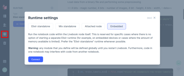
Then we were finally able to train our neural network on a GPU, achieving a significant training time improvements.

Conclusion

Although still in its early stages, machine learning in Elixir seems very promising. If you are familiar with ML and matrix manipulation libraries used in the world of Python, you will feel at home with Elixir. But, as noted, there are some things that require a bit of polishing. If you want to play with the data and livebooks containing the code presented in this article, we recommend you check out our

Git repository

.

At profiq, we are already using Elixir in production. We think the language is overall quite well- designed, and especially suited very well for high-traffic applications. The fact that ML libraries are being developed for this language as well is an additional feature that might help us and our clients easily extend their products with ML models.